LSTMs

\(\\)

LSTMs to Model Physiological Time Series

Harini Suresh, Nicholas Locascio, MIT

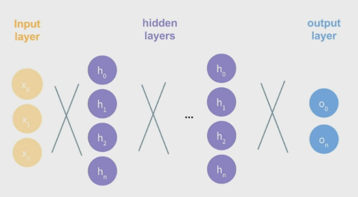
Neural Networks

\(\\)

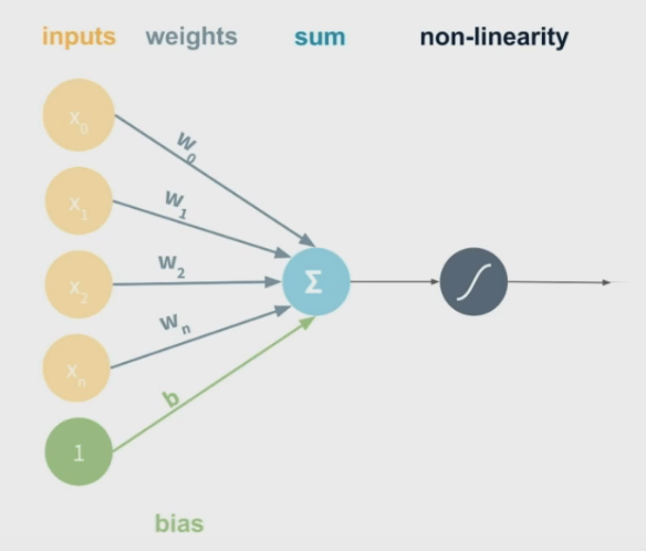
output of each node (perceptron) \(= g((\sum_{i=0}^{N} x_i * w_i )+b) = g(XW + b)\) (matrix notation)

\(\\)

These allow us to draw non-linear decision boundaries.

$$ loss \mathrel{\unicode{x2254}} J(\theta) = \frac{1}{N}\sum_{i}^{N}loss(f(x^{(i)};\theta),y^{(i)}))$$ where $\theta = W_1, W_2, ..., W_n$

Stochastic Gradient Descent (SGD)

• Initialize \(\theta\) randomly
• For N Epochs
  • For each training example \((x,y)\):
    • Compute loss gradient \(\frac{\partial J(\theta)}{\partial \theta}\)
    • Update \(\theta \mathrel{\unicode{x2254}} \theta - \eta \frac{\partial J(\theta)}{\partial \theta}\)

Example:

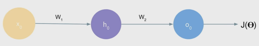
Using back-propagation and chain rule to calculate loss change with respect to a specific weight:

\(\\)

$with\ respect\ to\ W_2$

\[\frac{\partial J(\theta)}{\partial W_2} = \frac{\partial J(\theta)}{\partial o_0} * \frac{\partial o_0}{\partial W_2}\] i.e. how loss changes with output (multiplied by) how output changes with $W_2$

$with\ respect\ to\ W_1$

\[\frac{\partial J(\theta)}{\partial W_1} = \frac{\partial J(\theta)}{\partial o_0} * \frac{\partial o_0}{\partial h_0} * \frac{\partial h_0}{\partial W_1}\]

Recurrent Neural Networks (RNNs)

\(\\)

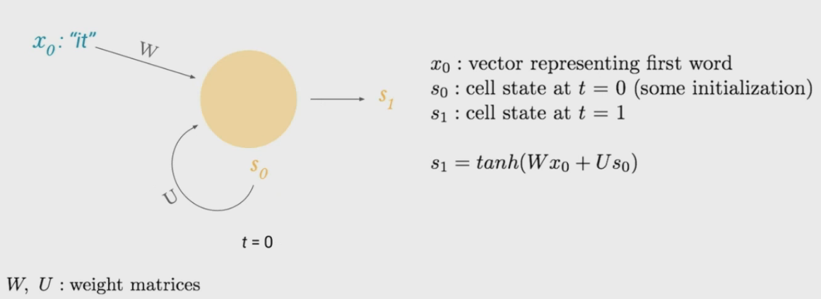
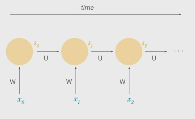
• Remembers previous state. Each hidden unit produces:
  • Function of input
  • Function of its own previous state/output
• Weights $W$ and $U$ stay the same across a sequence, so the model does not need to relearn something that applies later in a sequence
• $S_n$ can contain information from all past timesteps
• Benefit of Recurrent Neural Networks (over vanilla):
  • Maintains sequence order
  • Shares parameters across sequence so rules don’t need to be relearned
  • Keep track of long-term dependencies

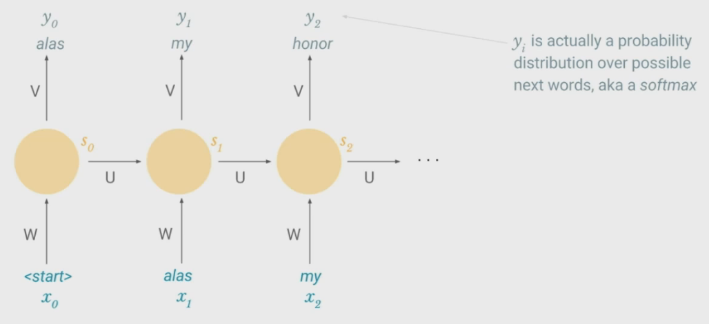
Possible Task - Language Model

\(\\)

• In addition to producing a state at each time, model produces an output (by multiplying another set of weights, $V$)
• Output is the probability distribution over the most likely next words, given what the network has seen before
• Loss function for training will measure similarity of output to training set

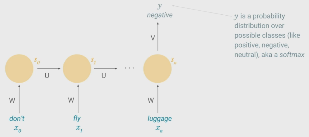
Possible Task - Sentiment Classification

\(\\)

• Output is probability distribution over possible classes (+/0/-)
• Network creates a representation of entire sequence and prediction is made based on cell state at last time step.

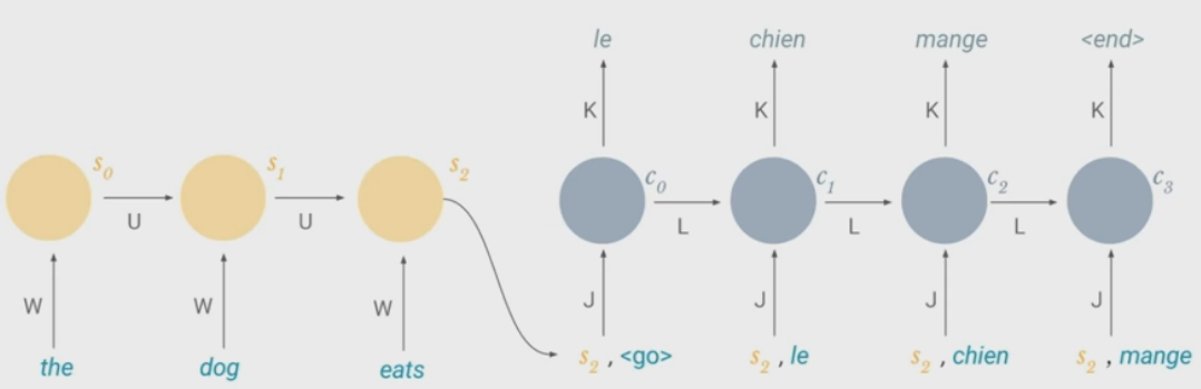
Possible Task - Machine Translation

\(\\)

• Made up of two RNNs
• Encoder takes a source sentence and feeds last cell state (encoded meaning of sentence) into second network
• Decoder produces output sentence in different language

Training RNNs - Backpropagation Through Time

\(\\)

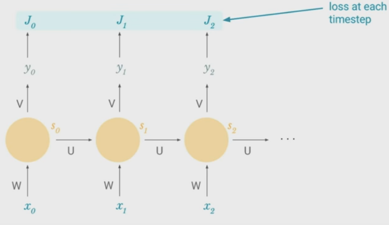
1. Take derivative (gradient) of loss with respect to each parameter
2. Shift parameters in the opposite direction of derivative to minimize loss

\[\frac{\partial J_2}{\partial W} = \sum_{k=0}^2 \frac{\partial J_2}{\partial y_2} \frac{\partial y_2}{\partial s_2} \frac{\partial s_2}{\partial s_k} \frac{\partial s_k}{\partial W}\]

At $k=0$, the third term in the summation, $\frac{\partial s_2}{\partial s_k} = \frac{\partial s_2}{\partial s_1} \frac{\partial s_1}{\partial s_0}$

The last two terms are the contributions of $W$ in previous time steps to the error at time step $t$

RNN Vanishing Gradient Problem

$$\frac{\partial s_n}{\partial s_{n-1}} = W^T diag[f'(W_{s_j - 1} + U_{X_j})]$$

• $W$ is sampled from a standard normal distribution, mostly $W<1$
• $f$ is $tanh$ or $sigmoid$, so $f’<1$
• As the gap between time steps get bigger, we multiply a lot of small numbers together
• Errors due to further back time steps have increasingly smaller gradients since we have to pass through a long chain rule for it to be counted in the loss. Parameters become biased to capture shorter-term dependencies

Solution 1 - Activation Functions

\(\\)

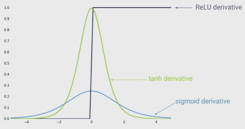
• ReLU derivative terms are not always less than 1 (unlike $tanh$ or $sigmoid$), so its derivatives will not contribute to shrinking the product

Solution 2 - Initialization

\(I_n = \begin{bmatrix}1 & 0 & 0 & \dots & 0\\0 & 1 & 0 & \dots & 0\\ 0 & 0 & 1 & \dots & 0\\ \vdots & \vdots & \vdots & \ddots & \vdots \\ 0 & ) & 0 & \dots & 1 \end{bmatrix}\)